이제 코드로도 짜봐야지

읽기 전에

지난 번 트랜스포머(Transformer) 논문 뽀개기에 이어, 코드 레벨로 구현해보았다.

이 포스트를 읽기 전에 아래의 두 포스트를 읽으면 도움이 될 것이다.

참조한 사이트

현청천 님의 블로그에 있는 코드들을 대부분 참고했다.

이 블로그에서 데이터는 Naver 영화리뷰 데이터를 사용해 Binary Classification으로 구현하셨다. 그런데 단순히 똑같이 따라하면 재미가 없으니, 나는 Multi-Label Classification으로 변경하면서, 예외처리를 조금 더 추가하는 방향으로 코드를 구현했다. 또한 모든 코드를 작성한 것이 아닌, 핵심 부분만 작성했으니 전체 코드를 보고 싶으면 위 참조 사이트를 가서 보면 된다.

정말 좋은 글 감사합니다!

트랜스포머 코드 구현

데이터 전처리 부분은 깔끔하게 스킵하겠다. 위 블로그를 접속하면 전처리를 어떻게 진행하는 지 확인할 수 있다.

임베딩

트랜스포머의 임베딩은 Input Embedding과 Positional Encoding 두 가지를 합쳐서 사용한다.

image-center

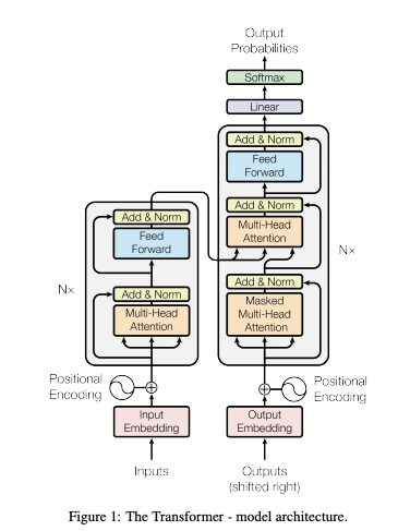
그림을 보면 인코더와 디코더 쪽에 모두 Input Embedding 과 Positional Encoding이 사용된다는 것을 확인할 수 있다.

Input Embedding

임베딩이란?

우리가 쓰는 단어들은 머신러닝 모델에 그대로 주입할 수 없다. 이미 알테지만, 학습을 한다는 것은 행렬과 벡터의 연산으로 가중치를 조절하는 것 이기 때문이다. 그렇기 때문에 입력시키는 무언가(예를 들면 단어, 문장 등 토큰)를 벡터로 변경시켜주는 작업이 필요하다. 이것이 바로 임베딩이다.

Input Embedding은 pytorch 내에서 사용되는 임베딩 함수를 그대로 활용하며, inputs에 대한 embedding 값 input_embs를 구한다.

n_vocab = len(vocab) # vocab count
d_hidn = 128 # hidden size
nn_emb = nn.Embedding(n_vocab, d_hidn) # embedding 객체

input_embs = nn_emb(inputs) # input embedding
print(input_embs.size())

Positional Embedding

트랜스포머는 sequence 순서를 사용하기 위해 토큰의 순서대로 상대적/절대적인 위치에 대한 정보를 반드시 주입해야한다 라고 했다. 그래야지만 단어의 순서를 파악할 수 있고, 정확한 값을 예측해낼 수 있기 때문이다.

이를 계산하는 방법은

\[\text{PE}_{(pos, 2i)} = sin(pos/10000^{2i/d_{model}}) \\ \text{PE}_{(pos, 2i + 1)} = cos(pos/10000^{2i/d_{model}})\]

라고 논문에서 설명했으니, 이를 코드로 옮겨보자!

먼저 Position Encoding을 구하는 방법이다.

각 포지션 별로 angle 값을 구한다(cal_angle)
구해진 angle들 중 짝수 index에는 sin함수를, 홀수 index에는 cos함수를 적용한다.

""" sinusoid position embedding """
def get_sinusoid_encoding_table(n_seq, d_hidn):
    def cal_angle(position, i_hidn):
        return position / np.power(10000, 2 * (i_hidn // 2) / d_hidn)
    def get_posi_angle_vec(position):
        return [cal_angle(position, i_hidn) for i_hidn in range(d_hidn)]

    sinusoid_table = np.array([get_posi_angle_vec(i_seq) for i_seq in range(n_seq)])
    sinusoid_table[:, 0::2] = np.sin(sinusoid_table[:, 0::2])  # even index sin 
    sinusoid_table[:, 1::2] = np.cos(sinusoid_table[:, 1::2])  # odd index cos

    return sinusoid_table

이를 그래프로 나타내면 다음과 같이 나타난다.

n_seq = 64
pos_encoding = get_sinusoid_encoding_table(n_seq, d_hidn)

print (pos_encoding.shape) # 크기 출력
plt.pcolormesh(pos_encoding, cmap='RdBu')
plt.xlabel('Depth')
plt.xlim((0, d_hidn))
plt.ylabel('Position')
plt.colorbar()
plt.show()

image-center

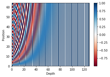
그래프에서 보이듯, 각 포지션 별로 다른 값을 갖는다는 것을 확인할 수 있다.

이제 Positional Encoding값을 가지고 Position Embedding 값을 구한다.

위에서 구해진 position encodong 값을 이용해 position emgedding을 생성합니다. 학습되는 값이 아니므로 freeze옵션을 True로 설정 합니다.
입력 inputs과 동일한 크기를 갖는 positions값을 구합니다.
input값 중 pad(0)값을 찾습니다.
positions값중 pad부분은 0으로 변경 합니다.
positions값에 해당하는 embedding값을 구합니다.

pos_encoding = torch.FloatTensor(pos_encoding)
nn_pos = nn.Embedding.from_pretrained(pos_encoding, freeze=True)

positions = torch.arange(inputs.size(1), device=inputs.device, dtype=inputs.dtype).expand(inputs.size(0), inputs.size(1)).contiguous() + 1
pos_mask = inputs.eq(0)

positions.masked_fill_(pos_mask, 0)
pos_embs = nn_pos(positions) # position embedding

print(inputs)
print(positions)
print(pos_embs.size())

이제 위에서 구한 input_embs와 pos_embs를 더하면 transformer에 입력할 input이 된다.

input_sums = input_embs + pos_embs

스케일드 닷-프로덕트 어텐션

image-center

\[\text{Attention}(Q, K, V = \text{softmax}(\frac{QK^T}{\sqrt{d_k}})V\]

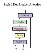
입력값

입력값은 Q(query), K(key), V(value) 그리고 attention mask로 이루어져 있다. 입력값 중 K, V는 같은 값이어야 한다(Q까지 같으면 셀프 어텐션이라고 한다).

계산 순서

계산 순서는 다음과 같습니다.

K 행렬 전치(transpose)
Q 와 K 전치행렬 MatMul
스케일 조절
마스킹(Mask)
Softmax
5번의 결과값과 V를 MatMul

Q = input_sums
K = input_sums
V = input_sums
attn_mask = inputs.eq(0).unsqueeze(1).expand(Q.size(0), Q.size(1), K.size(1))

attn_mask의 값은 pad(0) 부분만 True 입니다.

tensor([[False, False, False, False, False, False,  True,  True],
        [False, False, False, False, False, False,  True,  True],
        [False, False, False, False, False, False,  True,  True],
        [False, False, False, False, False, False,  True,  True],
        [False, False, False, False, False, False,  True,  True],
        [False, False, False, False, False, False,  True,  True],
        [False, False, False, False, False, False,  True,  True],
        [False, False, False, False, False, False,  True,  True]])

K-transpose and MatMul

앞서 적은 1번과 2번에 대한 코드입니다.

scores = torch.matmul(Q, K.transpose(-1, -2))

스케일

score에 k-dimension에 루트를 취한 값으로 나누는 코드다.

d_head = 64
scores = scores.mul_(1/d_head**0.5)

이 작업을 통해 가중치의 편차를 줄여줍니다.

마스킹

4번에 대한 코드이다.

scores.masked_fill_(attn_mask, -1e9)
print(scores.size())
print(scores[0])

mask를 한 부분이 -1e+9로 매우 작은 값으로 변경된다.

torch.Size([2, 8, 8])
tensor([[ 3.1348e+01, -1.4505e-01, -1.4832e+00, -2.8843e+00, -1.2542e+00,  8.3138e-01, -1.0000e+09, -1.0000e+09],
        [-1.4505e-01,  2.7846e+01,  4.9304e+00,  8.7807e-01,  1.5047e+00,  1.6372e+00, -1.0000e+09, -1.0000e+09],
        [-1.4832e+00,  4.9304e+00,  2.6831e+01,  3.9618e+00,  2.1587e+00,  3.5587e+00, -1.0000e+09, -1.0000e+09],
        [-2.8843e+00,  8.7807e-01,  3.9618e+00,  2.7904e+01,  1.6892e+00,  4.0453e+00, -1.0000e+09, -1.0000e+09],
        [-1.2542e+00,  1.5047e+00,  2.1587e+00,  1.6892e+00,  3.2076e+01,  4.0136e+00, -1.0000e+09, -1.0000e+09],
        [ 8.3138e-01,  1.6372e+00,  3.5587e+00,  4.0453e+00,  4.0136e+00,  3.8098e+01, -1.0000e+09, -1.0000e+09],
        [-5.7174e+00,  5.5846e-01,  3.0447e+00,  4.7429e+00, -1.1263e+00, -2.7216e+00, -1.0000e+09, -1.0000e+09],
        [-5.7174e+00,  5.5846e-01,  3.0447e+00,  4.7429e+00, -1.1263e+00, -2.7216e+00, -1.0000e+09, -1.0000e+09]],
       grad_fn=<SelectBackward>)

Softmax

5번에 대한 코드다

attn_prob = nn.Softmax(dim=-1)(scores)

이 코드를 통해 가중치가 확률로 변환된다. mask를 한 부분은 모두 0이 된다.

다시 한 번 MatMul

5번 attn_prob와 V를 MatMul하는 코드다.

context = torch.matmul(attn_prob, V)
print(context.size())

이렇게 계산하면 Q와 동일한 shape 값이 구해진다. 이 값은 V값들이 attn_prov의 가중치를 이용해서 더해진 값이다.

torch.Size([2, 8, 128])

차근차근 따라가면 눈에 잘 보일 것이다.

멀티 헤드 어텐션

image-center

\[\text{MultiHead}(Q, K, V) = \text{Concat}(\text{head}_1, \cdots, \text{head}_h)W^o \\ \text{where } \text{head}_i = \text{Attention}(QW^Q_i, KW^K_i, VW^V_i)\]

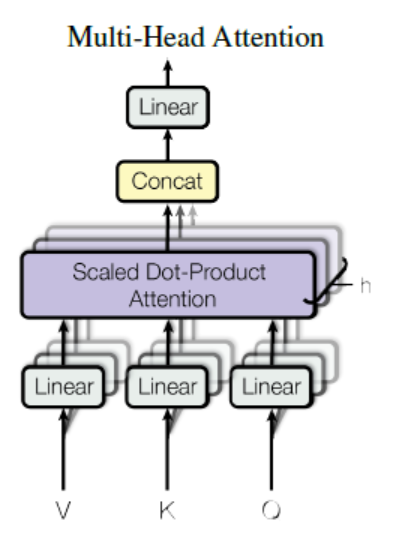
입력값

Q,K,V,atten_mask는 스케일드 닷-프로덕트 어텐션과 동일하다. head 개수는 2개 head의 dimension은 64다.

Q = input_sums
K = input_sums
V = input_sums
attn_mask = inputs.eq(0).unsqueeze(1).expand(Q.size(0), Q.size(1), K.size(1))

batch_size = Q.size(0)
n_head = 2

계산 순서

계산 순서는 다음과 같습니다.

Q, K, V를 여러 개의 Head로 나눈다(Multi-Head)
앞서 계산한 스케일드 닷-프로덕트 어텐션을 사용한다.
2번의 계산을 Concat해서 묶어준다.
Linear 계산을 해준다.

Multi Head Q,K,V

1번에 대한 계산입니다.

W_Q = nn.Linear(d_hidn, n_head * d_head)
W_K = nn.Linear(d_hidn, n_head * d_head)
W_V = nn.Linear(d_hidn, n_head * d_head)

# (bs, n_head, n_seq, d_head)
q_s = W_Q(Q).view(batch_size, -1, n_head, d_head).transpose(1,2)
# (bs, n_head, n_seq, d_head)
k_s = W_K(K).view(batch_size, -1, n_head, d_head).transpose(1,2)
# (bs, n_head, n_seq, d_head)
v_s = W_V(V).view(batch_size, -1, n_head, d_head).transpose(1,2)
print(q_s.size(), k_s.size(), v_s.size())

Q, K, V ahen Multi Head로 나눠졌습니다.

torch.Size([2, 2, 8, 64]) torch.Size([2, 2, 8, 64]) torch.Size([2, 2, 8, 64])

Attetion Mask도 Multi Head로 변경한다.

attn_mask = attn_mask.unsqueeze(1).repeat(1, n_head, 1, 1)

스케일드 닷-프로덕트 어텐션

위 결과에 스케일드 닷-프로덕트 어텐션을 계산한다.

scaled_dot_attn = ScaledDotProductAttention(d_head)
context, attn_prob = scaled_dot_attn(q_s, k_s, v_s, attn_mask)

Concat

위 결과물을 하나로 묶어주는 Concat 작업을 해준다.

context = context.transpose(1, 2).contiguous().view(batch_size, -1, n_head * d_head)
print(context.size())

Linear

마지막 Linear 작업이다.

linear = nn.Linear(n_head * d_head, d_hidn)
# (bs, n_seq, d_hidn)
output = linear(context)

마스킹된 멀티 헤드 어텐션

마스킹된 멀티 헤드 어텐션은 기존 멀티 헤드 어텐션과 attention mask를 제외한 모든 부분은 동일하다.

""" attention decoder mask """
def get_attn_decoder_mask(seq):
    subsequent_mask = torch.ones_like(seq).unsqueeze(-1).expand(seq.size(0), seq.size(1), seq.size(1))
    subsequent_mask = subsequent_mask.triu(diagonal=1) # upper triangular part of a matrix(2-D)
    return subsequent_mask


Q = input_sums
K = input_sums
V = input_sums

attn_pad_mask = inputs.eq(0).unsqueeze(1).expand(Q.size(0), Q.size(1), K.size(1))
print(attn_pad_mask[1])
attn_dec_mask = get_attn_decoder_mask(inputs)
print(attn_dec_mask[1])
attn_mask = torch.gt((attn_pad_mask + attn_dec_mask), 0)
print(attn_mask[1])

batch_size = Q.size(0)
n_head = 2

멀티 헤드 어텐션

멀티 헤드 어텐션과 동일하므로 위에서 선언한 멀티 헤드 어텐션을 바로 호출한다.

attention = MultiHeadAttention(d_hidn, n_head, d_head)
output, attn_prob = attention(Q, K, V, attn_mask)
print(output.size(), attn_prob.size())

피드포워드 네트워크

image-center

\[\text{FFN}(x) = \text{max}(0, xW_1 + b_1)W_2 + b_2\]

첫 번째 선형 변환: $f_1 = xW_1 + b_1$
ReLU: $f_2 = \text{max}(0, f_1)$
두 번째 선형 변환: $f_3 = f_2W_2 + b_2$

첫 번째 선형 변환

conv1 = nn.Conv1d(in_channels=d_hidn, out_channels=d_hidn * 4, kernel_size=1)
# (bs, d_hidn * 4, n_seq)
ff_1 = conv1(output.transpose(1, 2))

입력에 비해 hidden dimesion이 4배 커진 것을 확인할 수 있다.

torch.Size([2, 512, 8])

ReLU(or gelu)

원래는 ReLU를 사용하지만 GELU를 사용하는 것이 더 좋다고 알려졌다.

# active = F.relu
active = F.gelu
ff_2 = active(ff_1)

두 번째 선형 변환

conv2 = nn.Conv1d(in_channels=d_hidn * 4, out_channels=d_hidn, kernel_size=1)
ff_3 = conv2(ff_2).transpose(1, 2)
print(ff_3.size())

입력과 동일한 shape으로 변경된다.

torch.Size([2, 8, 128])

Multi-label Classification으로 변경

해당 블로그와 다르게 구현한 부분을 설명하기 위해 이 부분을 따로 뺐다.

단일 라벨에서 다중 라벨을 받을 수 있도록 변경

데이터 셋을 만드는 부분에서 기존 코드는 단순히 라벨을 추가만 해주었다.

self.labels.append(data["label"])

하지만 멀티 라벨에서는 한 문장에 라벨이 여러 개가 붙을 수 있기 때문에 라벨을 원-핫 인코딩해서 넣어주어야 한다.

labels_one_hot = np.zeros(len(APPEAL) - 1, )
label_list = [x.strip() for x in data["label"].split(',')]
for single_label in label_list:
    if single_label != "" and single_label != "0":
        idx = int(single_label) - 1
        labels_one_hot[idx] = 1

self.labels.append(labels_one_hot.tolist())

문장이 인코딩 시퀀스보다 길어서 임베딩 out of index 에러가 발생하는 경우

내가 학습시킨 데이터가 이런 경우에 걸렸다. 이를 방지하기 위해서 문장이 일정 길이보다 길면 잘라내는 코드를 추가했다.

self.sentences.append([vocab.piece_to_id(p) for p in data["doc"]])

이것을

max_len = 256
self.sentences.append([vocab.piece_to_id(p) for p in data["doc"]][:max_len])

으로 변경해주면 된다.

손실함수 변경

기존 단일 라벨 분류에서 쓰는 손실함수를 다중 라벨 분류에 맞게 변경해준다

# criterion = torch.nn.CrossEntropyLoss()
criterion = torch.nn.BCEWithLogitsLoss()

왜 BCEWithLogitsLoss()를 써야하는지 궁금하다면 이 블로그를 참조하면 도움이 된다.

정확도 체크

정확도 또한 계산하는 방식이 달라져야 한다.

""" 모델 epoch 평가 """
def eval_epoch(config, model, data_loader):
    matchs = []
    model.eval()

    threshold = 0
    n_word_total = 0
    n_correct_total = 0
    with tqdm(total=len(data_loader), desc=f"Valid") as pbar:
        for i, value in enumerate(data_loader):
            labels, enc_inputs, dec_inputs = map(lambda v: v.to(config.device), value)

    # 변경 전
    #         outputs = model(enc_inputs, dec_inputs)
    #         logits = outputs[0]
    #         _, indices = logits.max(1)

    #         match = torch.eq(indices, labels).detach()
    #         matchs.extend(match.cpu())
    #         accuracy = np.sum(matchs) / len(matchs) if 0 < len(matchs) else 0

    #         pbar.update(1)
    #         pbar.set_postfix_str(f"Acc: {accuracy:.3f}")
    # return np.sum(matchs) / len(matchs) if 0 < len(matchs) else 0

    # 변경 후
    outputs = model(enc_inputs, dec_inputs)
            logits = outputs[0]
            n_word_total += len(logits)
            for i in range(len(logits)):
                for j in range(len(logits[i])):
                    if logits[i][j] >= threshold:
                        logits[i][j] = 1
                    else:
                        logits[i][j] = 0

            correct = 0
            total = 0
            for d, a in zip(logits, labels):
                for i in range(len(d)):
                    if d[i] == a[i]:
                        correct += 1
                    total += 1

            accuracy = correct / total

            pbar.update(1)
            pbar.set_postfix_str(f"Acc: {accuracy:.3f}")

[Python, Pytorch] Attention is All You Need 코드 구현

목차

읽기 전에

참조한 사이트

트랜스포머 코드 구현

임베딩

Input Embedding

Positional Embedding

스케일드 닷-프로덕트 어텐션

입력값

계산 순서

K-transpose and MatMul

스케일

마스킹

Softmax

다시 한 번 MatMul

멀티 헤드 어텐션

입력값

계산 순서

Multi Head Q,K,V

스케일드 닷-프로덕트 어텐션

Concat

Linear

마스킹된 멀티 헤드 어텐션

멀티 헤드 어텐션

피드포워드 네트워크

첫 번째 선형 변환

ReLU(or gelu)

두 번째 선형 변환

Multi-label Classification으로 변경

단일 라벨에서 다중 라벨을 받을 수 있도록 변경

문장이 인코딩 시퀀스보다 길어서 임베딩 out of index 에러가 발생하는 경우

손실함수 변경

정확도 체크